Recursive Refinement
Recursive Refinement (RR) is an interpolation method that you can use to interpolate properties and create surfaces with smooth contours and trends. The method creates a grid around your input data and assigns values from the data points to the nodes of the grid in order to build the output surface.
The grid starts with a coarser resolution than the resolution of the surface you want to create. The coarse resolution is refined iteratively in order to reach the resolution of the output surface. It does this via an iterative process with three steps:
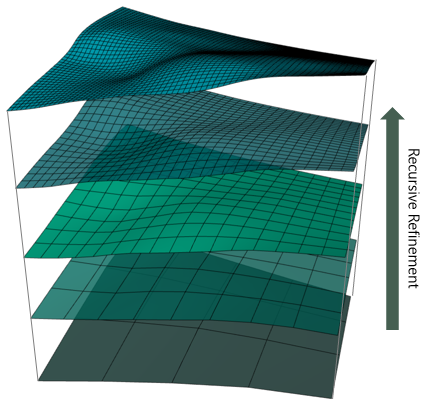
Recursive Refinement builds a surface in iterations. click to enlarge
- Snapping - the value of each input data point is assigned (snapped) to the nodes of the grid.
- Smoothing - a grid smoother function is applied to minimize the curvature of the surface.
- Refining - the cells of the grid are divided in half during each iteration.
Recursive Refinement is mainly steered by:
- The input data. In each iteration, the nodes of the grid are updated directly with values based on the input data and indirectly with information retrieved from the features of the surface that is under construction (e.g., derived direction, steepness, waviness etc.).
- The input settings. How coarse the initial grid starts and how many grid nodes receive a value in the first iteration play an important role in the end result (see the section Parameters for more detailed explanation).
The benefits of using this method are 1) the surface characteristics, as it produces surfaces with smooth contours, extrapolation and trends and 2) its usability, as it has very few input settings for which you can decide whether to have control over or interpolate with the defaults.
This interpolation method is available for selection in the workflows of Create Surface, Interpolate Property (prepare > Surfaces)
Procedure
To create a surface, Recursive Refinement initializes a grid around your input data. The nodes of the grid have initially no value. The method starts by snapping values from each input data point to the nearest grid nodes. A grid node can be affected by more than one input data point at the same time and for that reason a weighted average is used. This means that data points closer to a grid node have greater effect on the value that the node will receive. After the initial snapping, the nodes of the grid have received a value, forming an initial surface.
The grid is then smoothed and refined. The refinement process divides each grid cell in half, introducing new nodes to the existing grid and making the size of the grid cells smaller. From this stage onwards the method not only uses the input data, but also extra information from the grid slope and curvature to insert new grid nodes and update the values of the nodes.
The method repeats the processes of snapping, smoothing and refining until the final resolution is achieved. The final values are 'snapped' and tied to the grid nodes while the grid is smoothed one last time. The result is a surface with smooth contours and trends in the desired resolution.
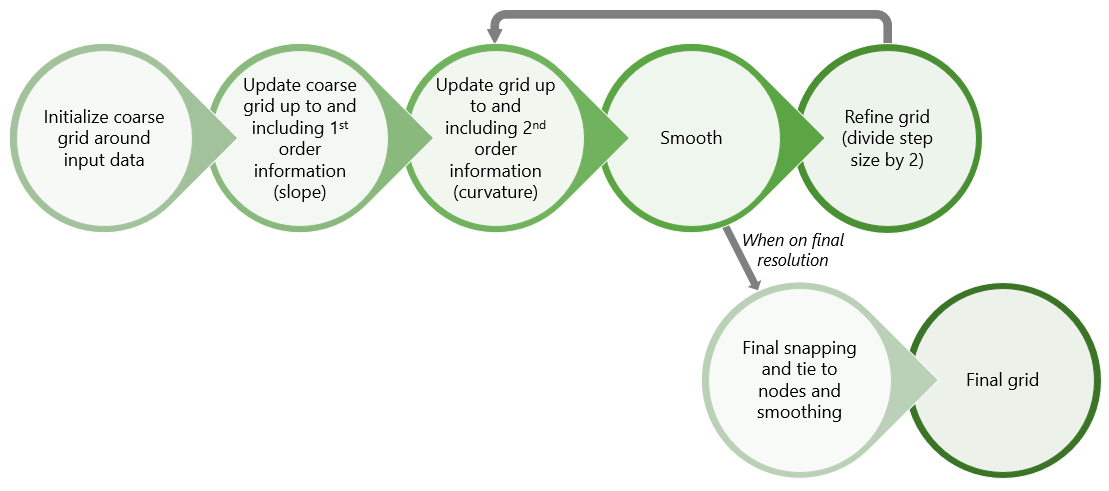
Recursive Refinement flow chart click to enlarge
Parameters
With Recursive Refinement (RR) you create a surface in iterations, by refining an initial coarse resolution in order to reach the final resolution. This means that the initial state has significant influence on the end result. For that reason, you have control over the initial grid, initial snapping and the final surface resolution. The iterations in-between are handled automatically with internal settings.
Initialization and Snapping
The workflow you use determines how the final grid resolution is specified. The initial grid resolution is based on the final resolution and the parameter Multiplier for initial coarse resolution. As the name implies, this is a number that is multiplied by the final resolution (X and Y increment) to produce the initial grid resolution. This parameter determines how coarse the initial grid will start relative to your final resolution and how many iterations need to be performed to reach the final resolution.
By default, the parameter Multiplier for initial coarse resolution is set to a value of 0 which means 'automatic'. In this case, Recursive Refinement determines the most suitable multiplier value for the initial grid resolution based on the requested final resolution and the distribution of your input data. The higher the value you enter for the multiplier, the coarser the initial grid will be.
With the parameter Grid nodes affected by snapping, you can determine the number of grid nodes that will be affected by each input data point in the first iteration. The default number is set to 16 grid nodes which means that each input data point will affect the nearest 16 grid nodes. This is also the maximum number possible (for more details on this parameters and why 16 is the maximum number, see the section below).
Recursive Refinement continuously updates the grid nodes with information from the input data. The 'Grid nodes affected by snapping' is the key parameter with which you can control how the input data influences those grid nodes.
- The example below shows one input data point (blue square) and a grid imposed on that point. The number of grid nodes that will be affected by snapping is set to 9. This means that the input data point will influence the 9 nearest grid nodes (yellow dots).
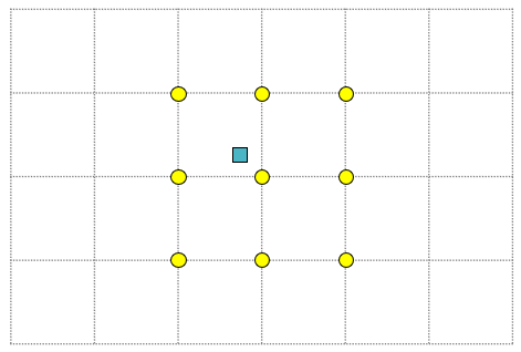
The input data point will affect 9 grid nodes in the imposed grid. click to enlarge
- This example shows two input data points (blue and green square) and a grid imposed on those points. The number of grid nodes that will be affected by snapping is still set to 9. In this case, the input data indicated with blue square will affect the nearest 9 grid nodes (yellow dots), while the input data indicated with green square will influence another 9 nearest grid nodes (red dots). There are, however, two grid nodes (orange dots with thick outline) affected by both input data points. The influence of each input data point on the final, combined value that these two grid nodes will receive, is determined with a weighting function.
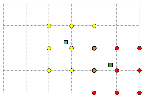
Each input data point will influence their nearest 9 grid nodes. A weighting technique is used to assign a value to the two grid nodes that are affected by both input data points. click to enlarge
Why the maximum is 16 grid nodes
Recursive Refinement uses a search box of 6 x 6 cells (7 x 7 nodes) around the input data to find the nearest grid nodes. For input data points that are not located near the edge of the interpolation area, the search box fits inside the area (left image below). In this scenario, all grid nodes inside the search box are valid nodes that could receive a value.
However, for input data points that are located near the edge of the interpolation area (right image below), the search box is partially outside that area. The nodes of the search box that are outside of the interpolation area cannot receive a value. The number of nodes found inside the interpolation area that can receive a value is at least 16. To ensure that each input data point affects the specified number of grid nodes within the interpolation area, the parameter 'Grid nodes affected by snapping' is maximized to 16 grid nodes (default setting).
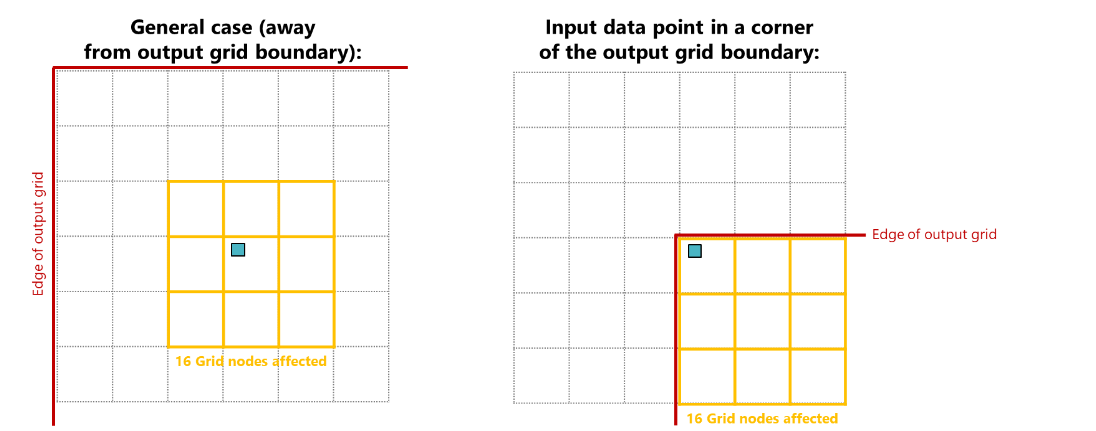
The parameter 'Grid nodes affected by snapping' is set to a maximum of 16 grid nodes. click to enlarge
Extrapolation
Recursive Refinement (RR) offers an extrapolation option to make sure that the entire surface receives values. In this way, you can handle cases of sparse or concentrated input data and/or insufficient parameter values (see Interplay between RR parameters for detailed explanation).
You can select to extrapolate in a linear way with the Extrapolation method 'Linear', or using a quadratic polynomial with the 'Quadratic' method. By default, the method is set to 'Linear' extrapolation. You can choose to not extrapolate by selecting the option 'None'.
If you choose to extrapolate, you also need to specify the Extrapolation area parameter. You can select between the options 'Outside convex hull' and 'As needed'. With 'Outside convex hull' the method starts to extrapolate directly outside the convex hull around your input data. With 'As needed' the method extrapolates in all areas where grid nodes are not receiving a value. By default the extrapolation area is set to 'As needed'.
Default settings
The table below shows an overview of the Recursive Refinement parameters with their default settings:
| Parameters | Defaults | Description |
|---|---|---|
| Multiplier for initial coarse resolution | 0 | automatically calculates the most suitable multiplier value |
| Extrapolation method | Linear | extrapolates using a linear function |
| Extrapolation area | As needed | extrapolates in areas without values |
| Grid nodes affected by snapping | 16 | each input data point affects the nearest 16 grid nodes |
Interplay between RR parameters
The final result depends heavily on the combination of your input data, the final resolution, the RR settings and your selection to extrapolate or not. Each parameter is designed to control a specific aspect of the process. In some cases, the combination of your settings can make some parameters to overrule others or have little to no effect on the end result (e.g., with a sufficiently high multiplier value, the grid receives values everywhere, making the specified extrapolation to have no effect on the end result). For that reason, Recursive Refinement requires some experimentation to discover what effect your parameters can have based on your input data and the area of interest.
Examples using Recursive Refinement
The examples below show how the RR parameters in combination with the given input data can affect the end result.
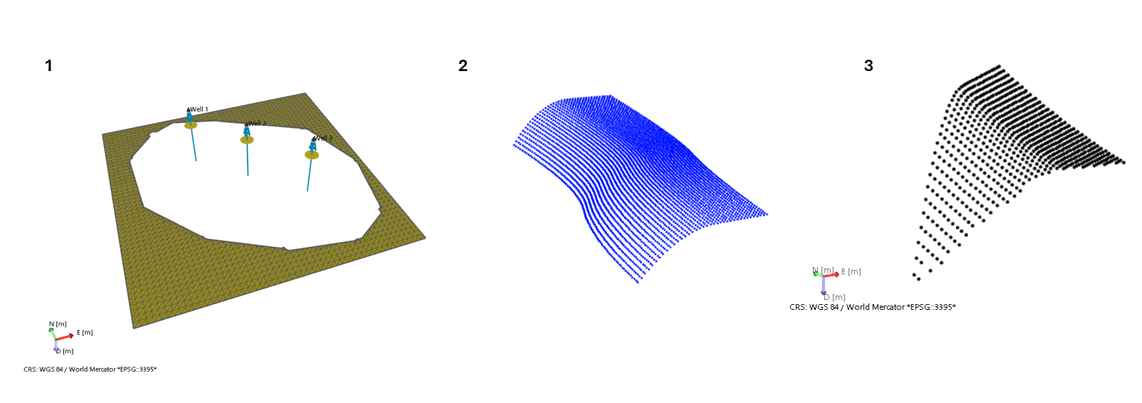
Three different input data were used for the below examples: 1) three markers at the center of the structure and some dense data in the outskirts, 2) gently dipping point set and 3) steeply dipping point set. click to enlarge
Example 1 Default settings
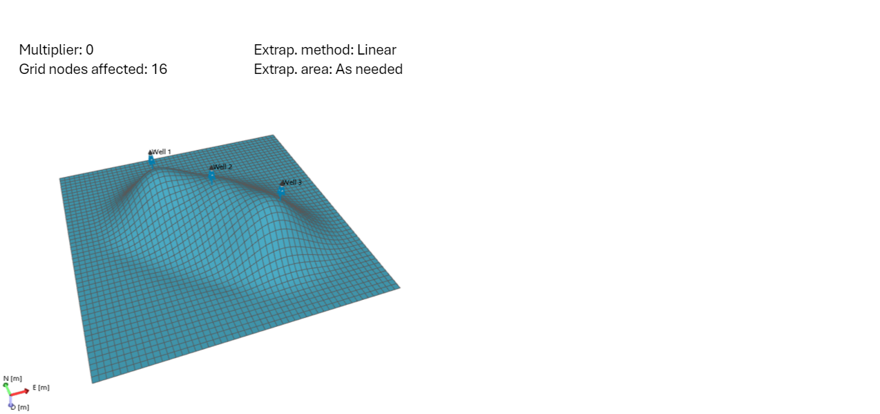
With the default settings, the initial grid resolution is automatically calculated by the method. It does this in the best way possible, such that extrapolation is used at a minimum. The input data is initially snapped to 16 grid nodes, which is the maximum number of nodes possible. This allows for a large coverage already from the first iteration. The extrapolation method 'Linear' ensures that all grid nodes receive a value. click to enlarge
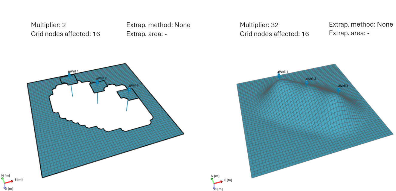
Example 2 Multiplier for initial coarse resolution
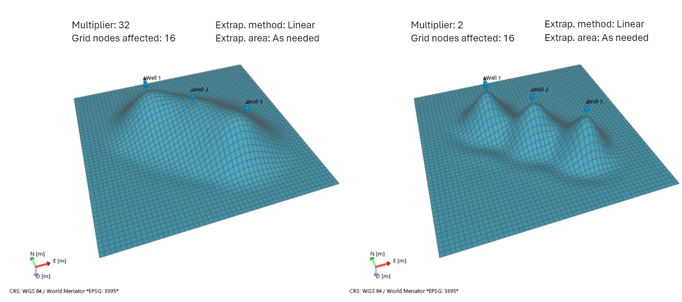
This example shows two output surfaces produced with different multiplier values. One is generated with a high multiplier value (left image) and one with a low multiplier value (right image). A high multiplier initialized a coarse grid resolution, while a low value initialized a finer initial grid resolution. For both surfaces the parameter 'Grid nodes affected by snapping' is set to the default value, which means that a large number of grid nodes received a value already form the initial snapping. The selection to extrapolate ensures that the entire surface is populated with values. The left combination of settings produces a 'bar' like surface, while the right a 'bull's eye' feature. click to enlarge
Example 3 Grid nodes affected by snapping
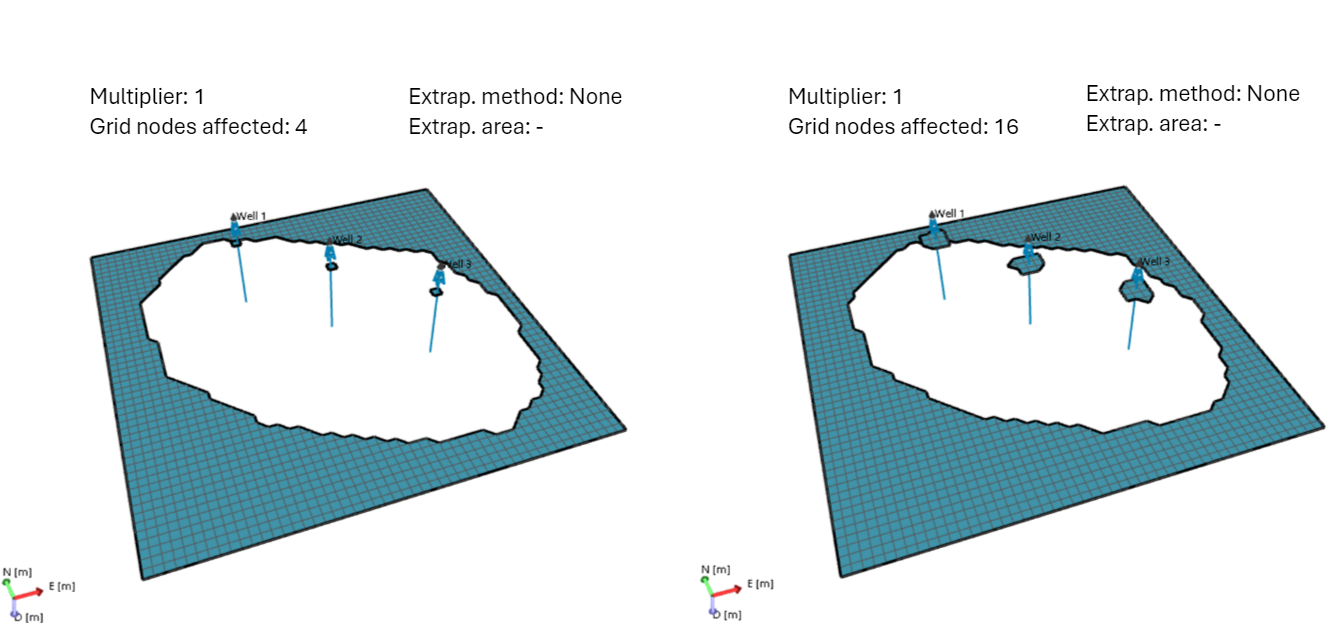
This example shows two output surfaces produced with different 'Grid nodes affected by snapping' values. One is generated with a low value (left image) and the other with the default value (right image). A low value means that a small number of grid nodes received a value during the initial snapping. A high value means that a large number of grid nodes received a value already from the initial snapping. The multiplier is set to a low number and the extrapolation to 'None', to show the effect of the main parameter in this example. click to enlarge
Example 4 Without Extrapolation
click to enlarge
This example shows two output surfaces generated without extrapolation. One surface is produced with a low multiplier (left image), while the other with a high multiplier (right image). The combination of settings in the left image leads to a 'patchy' surface since the initial grid is not coarse enough for RR to perform sufficient iterations and there is also no extrapolation to take care of the undefined grid nodes. The fact that the parameter 'Grid nodes affected by snapping' is set to the maximum of 16 grid nodes, it has little to no effect in this case. The combination of settings in the right image shows that even though there is no extrapolation, due to the high multiplier value and maximum number of grid nodes affected by snapping, the end surface is complete and smooth. click to enlarge
Example 5 Extrapolation method
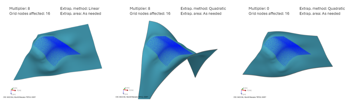
This example shows the effect of the two different extrapolation methods with i), ii) a low multiplier value (images left and middle) and iii) default multiplier value (right image). A low multiplier value can be insufficient for the method to populate with values the entire surface. For that reason, by selecting an extrapolation method you ensure that the entire output surface receives values. The surface on the left is created with 'Linear' extrapolation, while the one in the middle with 'Quadratic', which has a stronger effect on the end result. The right surface shows that when a high multiplier value is used (calculated by the method in this case), the extrapolation has no effect on the end result, since with a high multiplier the entire surface receives values from the input data. click to enlarge
Example 6 Extrapolation area
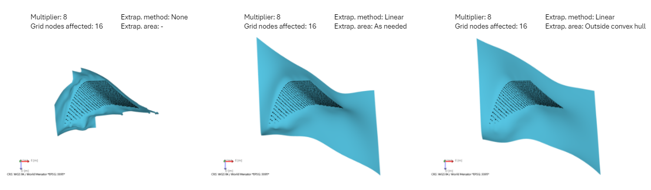
This example shows the effect of extrapolation on the output surface. The left image shows that when no extrapolation is selected, the method inherently extrapolates to a lesser extent. The image in the middle uses as extrapolation area 'As needed'. With this selection, any region outside the input data that does not receive a value, receives values with linear extrapolation. The image on the right uses as extrapolation area 'Outside convex hull' and as the name implies it starts to extrapolate directly outside the convex hull around the input data, resulting into a smoother transition right next to the data. click to enlarge